Using Linear Discriminant Analysis to classify image particles

This article describes, through a simple example, usage of a Linear Discriminant Analysis (LDA) technique to classify particles in an image.

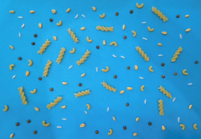
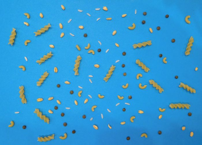
We start with a very simple, almost pre-segmented, image containing different kind of cereals : corn, rice, pasta shells, pasta torris and lentils :

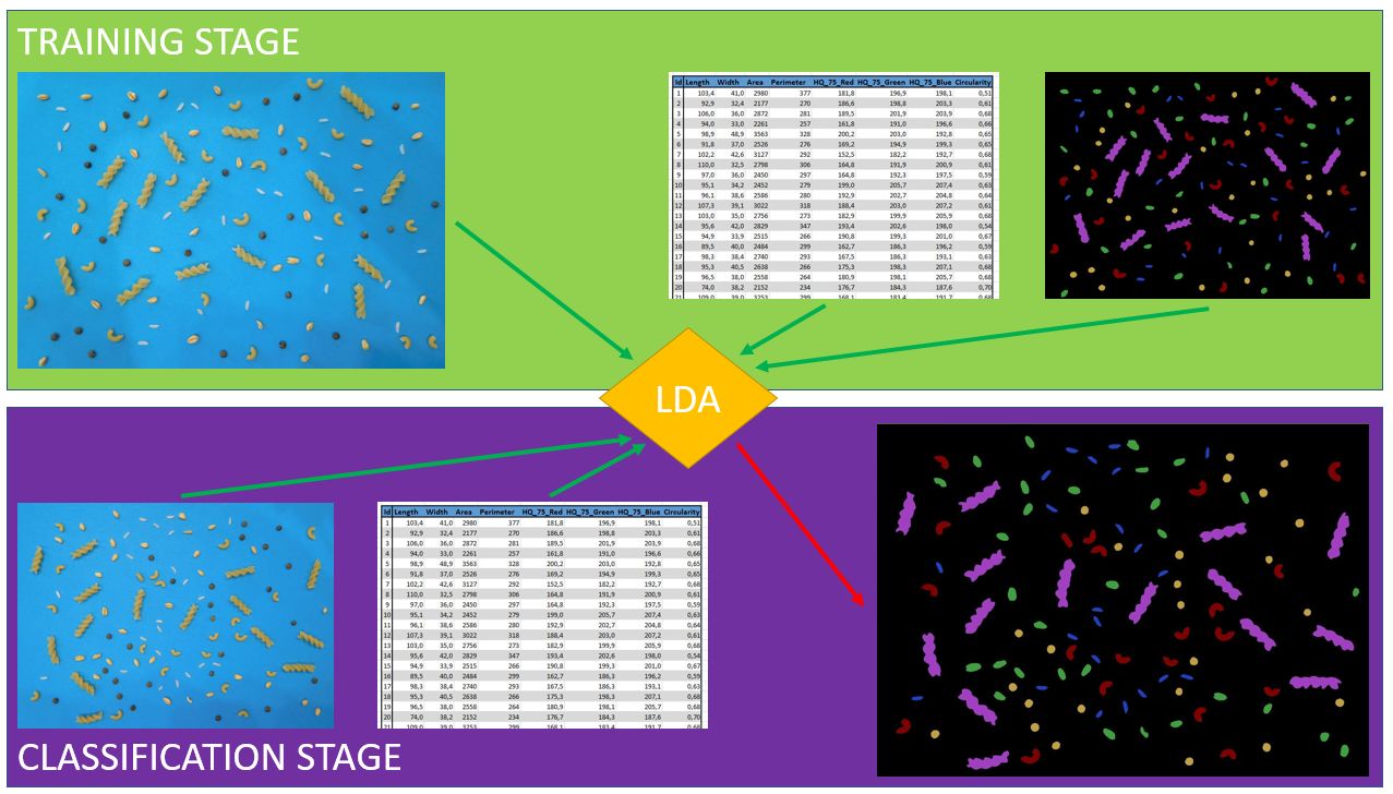
The aim of this method is to automatically (once a training stage proceeded) classify particles in an input image.

In the following we will present three main stages of such an algorithm :

define and extract measurements from input data
use some training data to reduce measurement space dimension and segment this sub space (LDA training stage)
classify some other data using previous results (LDA classification stage)

Note that LDA is usually defined as a dimensionality reduction algorithm but can also be used as a linear classifier algorithm (see here for an additional discution on this subject).

Definition and extraction of used measurements

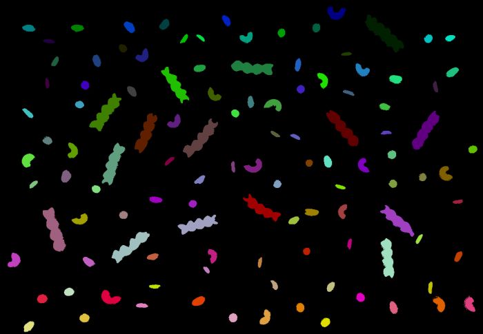
Since this image is almost segmented (ie particles are not in touch each other) we simply threshold image data and proceed to a connected component analysis to obtain an image where each particle has been assigned to a unique id (called a label) :

Using this last image as an overlay we get :

Since each particle area as been assigned to an unique id (label), we will then be able to proceed to some geometrical and photometric measurements for each particle :

geometrical measurements use a classical polygonal approximation of each particle boundary. Note that polygonal approximation will modify (simplify) particle boundary. This stage is usually based on a Douglas-Peucker algorithm.
photometric measurements use image intensities covered by each particle labeled area

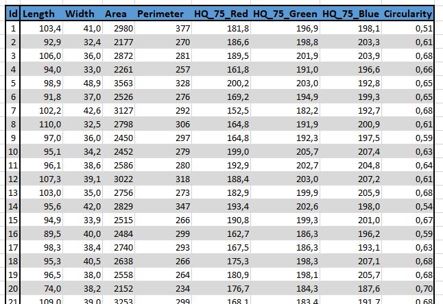
Here is a sample of such measurements which have been used in this example, for each particle we define :

[geometric] Length and Width obtained using an oriented bounding box algorithm.
[geometric] Area and Perimeter of each particule
[photometric] Histogram quantile at 75% point. Note that this measure is computed on each RGB channel of input image.
[geometric] Circularity defined as a combination of Area and Perimeter measurements

Applied to our input labeled image we are so able to compute associated measurements, getting information as the following :

LDA training stage

We saw in last part that we can associate some measurements to each identified particle in an input image. LDA training stage will consists in :

define list of such measurements and compute associated values for each particle
define classes for classification (here we define 5 different classes of cereals)
associate a class to each particle

These information will form training data for LDA algorithm.

As seen before, each particle has to be associated to a given class. We illustrate these handmade associations using a « label » image (each cereal class is represented with a different color) :

Once training data defined, LDA algorithm will « mix » input measurements and :

linearly combine input measurements to find the « best way » to separate each class given training data
reduce measurement space. Note that some input measurement may sometimes be discarded. This fact can be usefull when a lot of measurements are available and user doesn’t know which one to include in computation. Training step is usually an « offline » step which is allowed to take some processing time. In this case user can simply let LDA algorithm « choose » a subset of « usefull » measurements. Classification step will then be proceeded with this restricted subset of measurements.

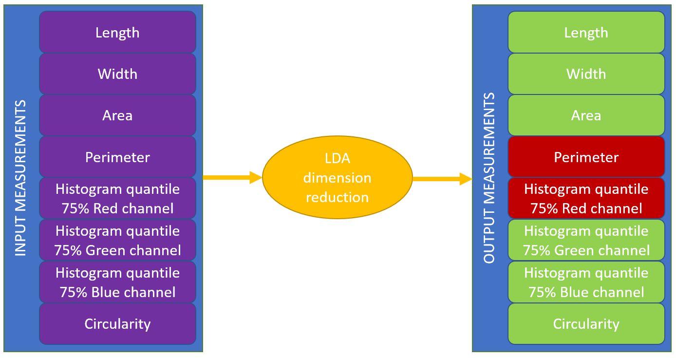
In our case, algorithm will form a linear combination which will allow to discard Perimeter and Histogram quantil on red channel from measurements set :

Note that in this article we focus on LDA algorithm usage leaving aside a lot of associated mathematical consideration (see here for more information). We nevertheless will give some additional information on classical pitfalls associated to this method in a next part.

LDA classification stage

In this stage we will consider new data that we want classify.

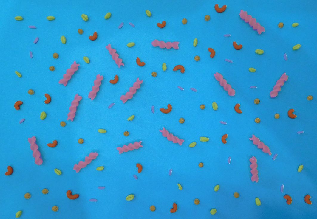
As in training stage case, we start with an « almost segmented » image (different from training image) :

And we proceed to a connected component analysis (in overlay) :

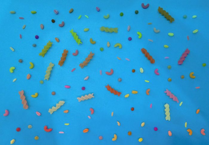
We will then compute the subset of measurements needed by LDA algorithm and obtain the following result applying classification stage of algorithm (each class is overlayed on input image) :

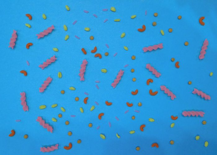
The following image illustrates this process :

LDA classical « pitfalls »

In the following we will present some (non exhausting) of the classical « pitfalls » associated to usage of LDA algorithm.

Statistical considerations

Mathematically, LDA algorithm works under a normal distribution assumption of the dataset (a multi normal distribution assumption in fact). Note that LDA algorithm has shown a great robustness toward this criterion but will perform in a weaker manier if input data are significantly non gaussian.

Measurements considerations

In a previous part we have seen that we can use LDA algorithm to reduce measurements space dimension and even in some case to discard some of then. This fact allows user to provide a lot of different measures to LDA algorithm letting it choose which measurements should be « used ».

Note that a classical « pitfall » in this field would consists in providing measurements which efficiently allows to classify training dataset but which are not the reflect of a standard population behavior.

A first geometrical example would be a case where we would have put all rice grains on the left part of training image, adding in the same time the barycenter coordinates of each particules to the measurements list. In this case an efficient manier for LDA algorithm to classify rice grain would then be to use X coordinates of barycenter of these paarticules.

A second photometric example could apply directly to our example in the case where some lighting condition may vary between training and classification acquisition. In this case the photometric measurements used by LDA algorithm (Histogram quantiles on green and blue channels) may become invalid between these two steps. A classical way to avoid this kind of problems consists in preprocessing input images using an histogram equalization algorithm.